How to detect Credit Card Fraud Using Python Pandas

 Detecting fraud in credit card transactions is an important application of Machine Learning.

Given below is a step-by-step guide on how to approach fraud detection using Python (Pandas and Scikit-Learn) with the Credit Card Fraud Detection Dataset from Kaggle:

Data source: Credit Card Fraud Detection Dataset https://www.kaggle.com/mlg-ulb/creditcardfraud

Step 1: Data Preprocessing

Start by importing the necessary libraries and loading the dataset into a Pandas DataFrame.

import pandas as pd

# Load the dataset
data = pd.read_csv('creditcard.csv') #replace with the downloaded file path# Explore the dataset
print(data.head())

Output:

Step 2: Data Exploration

Understand the dataset by checking its structure, summary statistics, and class distribution (fraudulent vs. non-fraudulent transactions).

# Check the dataset shape
print(data.shape)
# Check summary statistics
#print(data.describe())
# Check class distribution
print(data['Class'].value_counts())

Output:

(284807, 31)

0    284315
1       492
Name: Class, dtype: int64

Step 3: Data Splitting

Split the dataset into training and testing sets to evaluate the model’s performance.

from sklearn.model_selection import train_test_split

X = data.drop('Class', axis=1)  # Features
y = data['Class']  # Target variableX_train, X_test, y_train, y_test = train_test_split(X, y, test_size=0.2, random_state=42)

Step 4: Model Training

Train a machine learning model, such as Logistic Regression, on the training data.

from sklearn.linear_model import LogisticRegression

# Create a Logistic Regression model
model = LogisticRegression()# Fit the model to the training data
model.fit(X_train, y_train)

Output:

LogisticRegression()

Step 5: Model Evaluation

Evaluate the model’s performance on the test data using appropriate metrics such as accuracy, precision, recall, and F1-score.

from sklearn.metrics import classification_report, confusion_matrix

# Predict on the test data
y_pred = model.predict(X_test)# Evaluate the model
print("Confusion Matrix:")
print(confusion_matrix(y_test, y_pred))print("\nClassification Report:")
print(classification_report(y_test, y_pred))

Output:

Step 6: Visualizations

1. Confusion Matrix Heatmap

To draw a visual comparison between the predicted values and actual values for a binary classification problem like fraud detection, you can create a confusion matrix heatmap or a ROC curve.

Here’s how you can create a confusion matrix heatmap:

#Import the required libraries
import matplotlib.pyplot as plt
import seaborn as sns
from sklearn.metrics import confusion_matrix

# Calculate the confusion matrix
conf_matrix = confusion_matrix(y_test, y_pred)# Create a heatmap for the confusion matrix
plt.figure(figsize=(8, 6))
sns.heatmap(conf_matrix, annot=True, fmt="d", cmap="Blues", cbar=False,
            xticklabels=["Predicted 0", "Predicted 1"],
            yticklabels=["Actual 0", "Actual 1"])
plt.xlabel('Predicted')
plt.ylabel('Actual')
plt.title('Confusion Matrix')
plt.show()

Output:

Explaining this code:

• y_test represents the actual values (ground truth) from the test dataset.
• y_pred represents the predicted values from the model.

This code creates a heatmap where the x-axis represents the predicted classes (0 and 1 for non-fraud and fraud, respectively), and the y-axis represents the actual classes. The numbers inside the heatmap cells indicate the count of observations falling into each category. This visualization allows you to easily compare predicted and actual values and see how well your model is performing in terms of true positives, true negatives, false positives, and false negatives.

2. ROC curve

To show a Receiver Operating Characteristic (ROC) curve for the credit card fraud detection model, you can use Python libraries like matplotlib and sklearn.

import matplotlib.pyplot as plt
from sklearn.metrics import roc_curve, roc_auc_score, auc
from sklearn.model_selection import train_test_split
from sklearn.linear_model import LogisticRegression

#Train a logistic regression Model and predict with the model
X_train, X_test, y_train, y_test = train_test_split(X, y, test_size=0.2, random_state=42)
model = LogisticRegression()
model.fit(X_train, y_train)
y_pred = model.predict(X_test)
y_prob = model.predict_proba(X_test)[:, 1]

# Calculate ROC curve
fpr, tpr, thresholds = roc_curve(y_test, y_prob)# Calculate AUC (Area Under the Curve)
roc_auc = auc(fpr, tpr)# Plot ROC curve
plt.figure(figsize=(8, 6))
plt.plot(fpr, tpr, color='darkorange', lw=2, label=f'ROC curve (AUC = {roc_auc:.2f})')
plt.plot([0, 1], [0, 1], color='navy', lw=2, linestyle='--')
plt.xlim([0.0, 1.0])
plt.ylim([0.0, 1.05])
plt.xlabel('False Positive Rate')
plt.ylabel('True Positive Rate')
plt.title('Receiver Operating Characteristic (ROC) Curve')
plt.legend(loc='lower right')
plt.show()

Output:

Explaining this code:

• y_test represents the actual labels (ground truth) from the test dataset.
• y_prob represents the predicted probabilities of class 1 (fraudulent) from the model.

The code calculates the ROC curve and the Area Under the Curve (AUC) score and then plots the ROC curve. The ROC curve shows the trade-off between the true positive rate (TPR) and the false positive rate (FPR) as we vary the decision threshold. A higher AUC indicates better model performance.

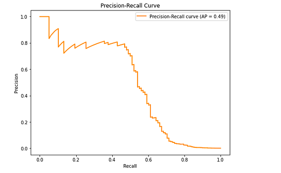
3. Precision Recall Curve

To show a Precision-Recall curve for the credit card fraud detection model, we can use Python libraries like matplotlib and sklearn.

import matplotlib.pyplot as plt
from sklearn.metrics import precision_recall_curve, average_precision_score
from sklearn.model_selection import train_test_split
from sklearn.linear_model import LogisticRegression

# Calculate Precision-Recall curve
precision, recall, thresholds = precision_recall_curve(y_test, y_prob)# Calculate Average Precision (AP)
average_precision = average_precision_score(y_test, y_prob)# Plot Precision-Recall curve
plt.figure(figsize=(8, 6))
plt.plot(recall, precision, color='darkorange', lw=2, label=f'Precision-Recall curve (AP = {average_precision:.2f})')
plt.xlabel('Recall')
plt.ylabel('Precision')
plt.title('Precision-Recall Curve')
plt.legend(loc='best')
plt.show()

Output:

Explaining this code:

• y_test represents the actual labels (ground truth) from the test dataset.
• y_prob represents the predicted probabilities of class 1 (fraudulent) from the model.

The code calculates the Precision-Recall curve and the Average Precision (AP) score and then plots the curve. The Precision-Recall curve shows the trade-off between precision and recall as we vary the decision threshold. A higher AP indicates better model performance.

Step 8: Fine-Tuning and Optimization

You can further optimize the model by fine-tuning hyperparameters, trying different algorithms (e.g., Random Forest, Gradient Boosting), and dealing with class imbalance using techniques like oversampling or undersampling.

Once you have a well-performing model, you can deploy it to a production environment for real-time fraud detection. This may involve setting up an API or integrating it into your payment processing system.